Known issues & methods!

What is this site?

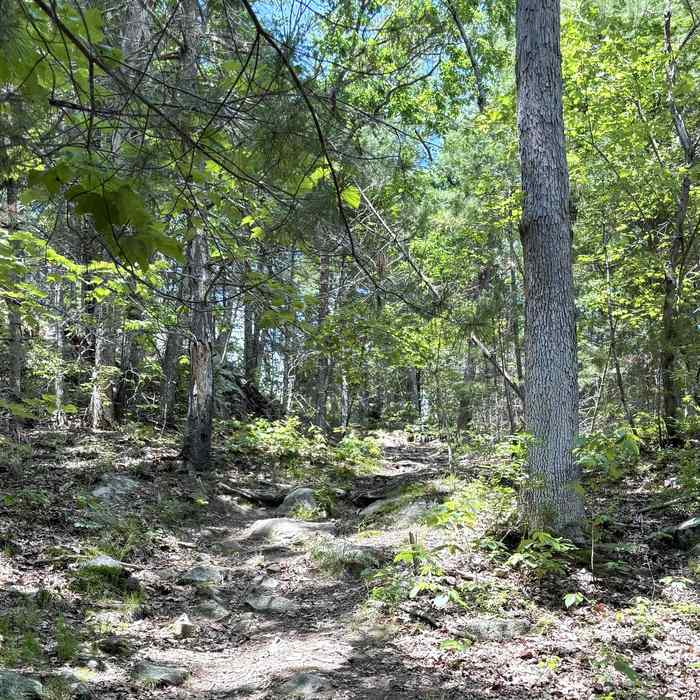
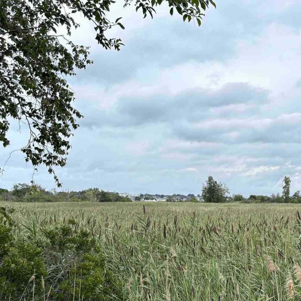
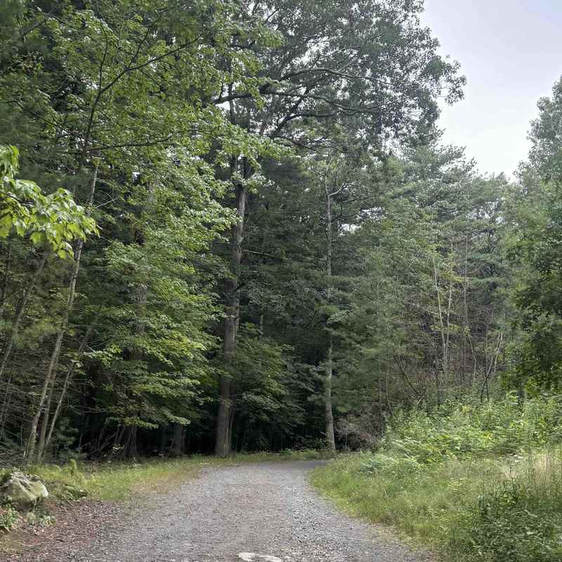
• I live in a city and really enjoy walking/hiking/running in the parks around the area. I really just wanted to figure out which parks around me were more likely to have “wild vibes” and go to them.

• At the same time though, this site also answers the question of who on Strava has been to the most remote point in the US (I’m now pretty sure it’s Arrigetch Peaks in AK).

• To calculate this, the US is divided up into >700 million hexagons using Uber’s H3 geospatial index. Isolation/remoteness is then measured by the shortest number of hexagons that must be traversed to reach a hexagon with a driveable road.

I also wasn’t aware when making this that:

1. a similar feature exists on GAIA GPS (but it also seems that this feature does not have resolution beyond 2 mi of isolation)

2. most remote spots within the largest wilderness complexes in the US had already been reported and calculated using a largest inscribed circle technique on Peakbagger.

Known issues!

1. OSM annotations

   • Tracks are not included as driveable roads: The OSM tag “track” has a very broad definition that includes many hiking paths as well as unpaved roads. Tracks were not considered driveable roads in this analysis, but this also means that offroad tracks can come quite close to some isolation points. This is common on beaches where oversand driving is permitted.

   • Misannotation of remote ways: Some remote ways are incorrectly classified as driveable. See the examples on Isle Royale, MI, and Loggerhead Key, FL. This can significantly skew the result, causing the actual state isolation point to be located further away and often in a different location.

2. H3 cells and orientations

   • H3 hexagons of the same resolution can vary up to two-fold in area: Issues with this are described very well in the docs for another geospatial index A5. I believe this makes it so that any one-dimensional distance calculated using these cells can be wrong by up to 20%. (Note that this could be fixed by including the edge length of each cell in the BFS but that’s too much work for now).

   • Hexagon orientation bias: Hexagons are obviously not equidistant from their center to any edge, and as a result distances can be slightly different depending on the direction in which they are measured. This is why you see isolated areas rotating around when crossing zoom levels that change cell resolutions.

Methods

Part of this project was an excuse to get familiar with AI agents. I used Cursor’s six-month Pro+ student trial, which was an insane deal.

1. Making SQL databases for ways

   • Geofabrik provides daily OpenStreetMap extracts in the .osm.pbf format for regions and subregions around the globe. I initially downloaded only the US region, but this would be incorrect near borders where a point could be closer to a road in Canada or Mexico than in the US.

   • Instead, a 100 km dilation was performed on the state shapefiles from the US Census (200 km for AK and HI) using an AEQD projection centered at the centroid of each state. Geofabrik extracts from all regions intersecting this dilated geometry were used:

     us-260721.osm.pbf
     canada-260817.osm.pbf
     mexico-260817.osm.pbf
     bahamas-260817.osm.pbf
     far-eastern-fed-district-260817.osm.pbf #russia
     

   • For each OSM file above, a separate PostgreSQL database was created with:

     osmium tags-filter REGION-DATE.osm.pbf w/highway -o REGION_ways.osm.pbf
     osm2pgsql -E 4326 -S default_plus_motor_vehicle.style -d REGION REGION_ways.osm.pbf
     

     Here, default_plus_motor_vehicle.style is based on the default from osm2pgsql, with the following line added because the motor_vehicle tag is not included automatically:

     node,way   motor_vehicle     text         linear
     

2. Converting road positions to H3 cell IDs

   • Ways must be filtered into driveable roads, segmentized into discrete points, and converted into unique H3 cell IDs. Surprisingly, this can be done with a single SQL command that runs relatively quickly:

     \copy (
         SELECT DISTINCT
             h3_latlng_to_cell(POINT(ST_X((dp).geom), ST_Y((dp).geom)), 10) AS h3_cell
         FROM planet_osm_line,
              ST_DumpPoints(ST_Segmentize(way::geography, 10)::geometry) AS dp
         WHERE COALESCE(area, '') NOT IN ('yes')
         AND COALESCE(access, '') NOT IN ('private')
         AND highway NOT IN ('abandoned', 'bridleway', 'bus_guideway', 'construction', 'corridor',
           'cycleway', 'elevator', 'escalator', 'footway', 'no', 'path', 'pedestrian', 'planned', 'platform',
           'proposed', 'raceway', 'razed', 'rest_area', 'services', 'steps', 'track')
         AND COALESCE(motor_vehicle, '') NOT IN ('no')
         AND COALESCE(motorcar, '') NOT IN ('no')
         AND COALESCE(service, '') NOT IN ('emergency_access', 'parking', 'parking_aisle', 'private')
     ) TO 'REGION_road_cells.csv' WITH CSV HEADER;
     

     In this command:

     • WHERE... is a filter for driveable roads that comes directly from the “drive_service” filter in OSMnx.

     • FROM... takes each road and segmentizes it into points spaced 10 m apart.

     • SELECT... finds the resolution 10 H3 cell containing each point, while DISTINCT removes duplicate cells.

   • The .csv files for each region are then merged with cat and made into a unique set with sort -u. The output is a list of all cells that contain roads in and near the US, 2 GB.

3. Calculating isolation distances

   • A list of all unique resolution 10 cells in the dilated US geometry was first obtained by running h3.geo_to_cells() on tiles that intersect the geometry and removing duplicates with sort -u, 17 GB.

   • A Google Cloud Compute Engine instance, c4a-highmem-16 with 128 GB memory and 100 GB Hyperdisk, was rented for ~$1/hr to run essentially nx.multi_source_dijkstra_path_length(), with road_cells.csv as the sources and neighbors given by h3.grid_disk(cell, 1). AI also thankfully wrote BFS using deque() without NetworkX to fit in memory. The output, named dist.csv, has cell IDs as the index and a single distance column, 20 GB.

   • This script was also run at every H3 resolution below 10, using h3.cell_to_parent(cell, NEW_RESOLUTION) to convert each node and source to the new resolution. In all, the cloud cost <$8.

4. Visualizing with MapLibre and PMTiles

   • For each resolution, dist.csv was converted to a .geojson. Each cell boundary was generated with h3.cell_to_boundary(cell), and the distance was saved as an attribute of the corresponding feature. Also only cells within the undilated US geometry were kept for visualization. For resolution 10, the .geojson was 136 GB.

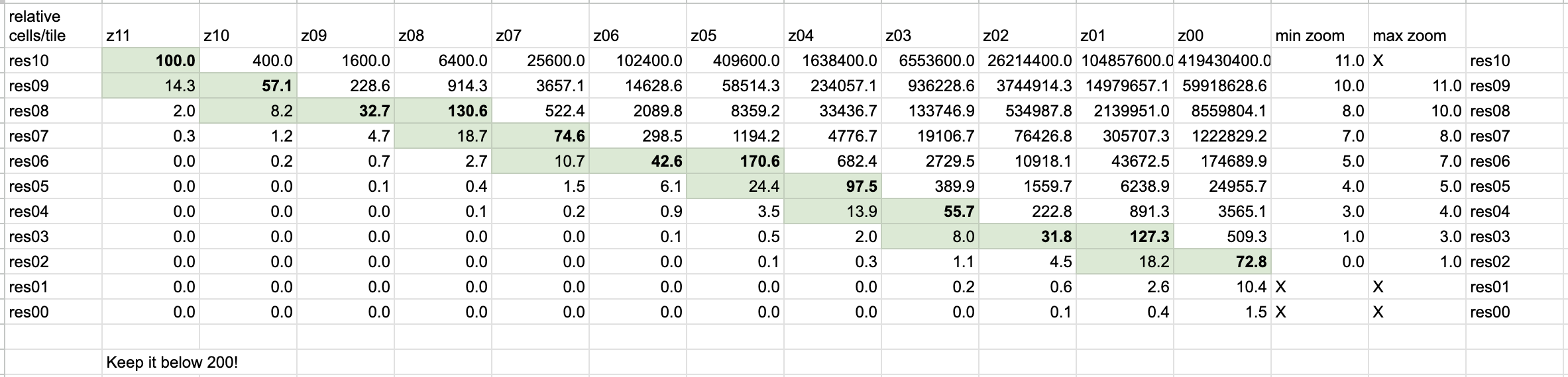
   • To keep the map working at lower zoom levels, lower resolution cells are displayed as the user zooms out. To limit the number of features shown at any given zoom level, each .geojson was converted to PMTiles only for a selected zoom range. The ranges in the table were chosen to keep the relative number of displayed features reasonably consistent.

   

   • Each .geojson was converted to PMTiles using Tippecanoe. The following resolution 10 example produces an 8 GB .pmtiles:

     tippecanoe -Z11 -z11 -t tmp -o res10_z11.pmtiles -l cells res10.geojson
     

   • In MapLibre, the .pmtiles for each resolution is referenced separately. Network distances are converted to miles using the average H3 edge length multiplied by √3, which gives the distance between adjacent hexagonal cell centers.